B-Splines
This page describes how to use B-splines in FreeCAD. It gives also background information what B-splines are and for what applications they are useful.
Motivation
If you know already about B-splines and their application, you can directly continue with section B-splines in FreeCAD.
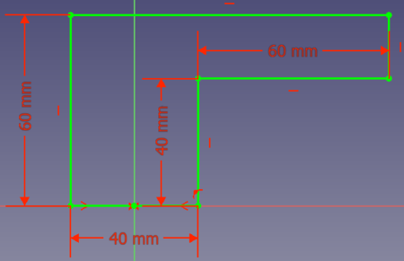
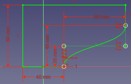
Let's assume you want to design a part that should be produced with a 3D printer. The part must have an edge this way:
You have to print the part in direction of the sketch's bottom to the top. Outer support structures might not be an option. Therefore you need to add a support directly to your part. What options do you have?
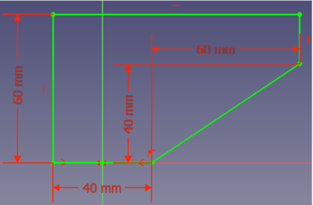
- Option 1: you could add a line from point (20, 0) to point (80, 40):
However this solution needs a lot of volume, thus weight and material.
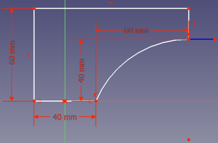
- Option 2: you can connect the two points with an arc of a circle. To save volume, the arc should end tangentially in point (80,40). Then your solution looks like this:
OK. But at the bottom you don't need immediate support.
- Option 3: you could save some more volume if the connection between the 2 points is a curve that begins tangentially at (0, 20) and ends tangentially at (80, 40):
So a curve with which you can connect two points tangentially to a reference point can be very useful for constructions. Bézier curves provide this feature.
Bézier curves
Derivation
Bézier curves are polynomials to describe the connection between 2 points. The simplest polynomial connecting 2 points is a line () thus linear Bézier curves are also line segments:
Animation 1: Linear Bézier curve.
However a polynomial becomes useful when we can control it. So there should be a point between the 2 endpoints that allows us to define how the endpoints are connected. Like in the above example option 3 the curve is helpful when it starts and ends tangentially to lines crossing the endpoints. And this is a main feature of Bézier curves. So let's add a control point between the 2 endpoints. The curve will start tangentially towards this control point, meaning it is tangential to the line that we can draw between the startpoint and the control point. Going backwards from the endpoint the curve will also be tangential to the line we can draw between the control point and the end point. Animation 2 shows how such a curve looks.
Animation 2: Quadratic Bézier curve. P1 is hereby the control point.
The animation makes clear what the curve basically is - a transition from P0 to P2 by rotating the line P0-P1 to become the line P1-P2. Therefore we get the nice tangential start/end feature.
Such a curve can only be described by a quadratic polynomial. (The number of left-hand/right-hand turns + 1 is the necessary polynomial order. A quadratic polynomial is a single turn, a cubic polynomial has two turn, and so on.) Therefore a Bézier curve with one control point is a quadratic (second order) Bézier curve.
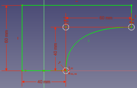
Having only one control point is often not sufficient. Take the above motivation example. There in option 3 we end the curve tangentially in x-direction. But how can you connect the points (20, 0) and (80, 40) so that the curve ends tangentially in y-direction? To achieve this you need first a right-hand and then a left-hand turn, so a cubic (third order) polynomial. And that means for a Bézier curve that we need (or you can say we gain) a second control point. Animation 3 shows a cubic Bézier curve.
Animation 3: Cubic Bézier curve.
To answer the question, the solution with the tangential y-direction ending for the example is this one:
Math
If you are interested to understand the background math, here are the basics.
A Bézier curve is calculated using this formula:
n is hereby the degree of the curve. So a Bézier curve of degree n is a polygon with order n. The factors are hereby in fact the coordinates of the Bézier curves' control points. For a visualization see Controlling Bézier curvatures.
If you are further interested, have a look at The mathematics of Bézier curves with a nicely animated derivation of the math of Bézier curves.
Basis
There is another way to view the mathematical expression. Each coordinate of a point on the curve can be seen as a polynomial function. Then, these polynomials can be described as a linear combination of polynomials , with the x/y coordinate of each of the control points as a factor. It can be shown that these particular sets of polynomials can describe any polynomial of degree with the right factors. These polynomials are then said to form a "basis" for all Bezier curves of degree .
These particular polynomials are called Bernstein polynomials. They have some interesting properties. (This part of the wiki is WIP)
A set of Bernstein polynomials with order 4. They describe a 4th order B-spline with 5 control points.
Rational Bezier Curves
Sometimes we want some curves to be closer to certain control points that to others. This can be done by applying "weights" to control points, and defining a new interpolation.
(WIP: Equation(s) go(es) here)
The denominator is added to ensure that the convex hull property is maintained. Notice the expression is now not a polynomial function of the parameter {t} anymore, but rational functions. Because of this, such curves are called Rational Bezier curves.
An interesting thing about rational Bezier curves is that they can now be used to exactly represent arcs of circles and other conics. (This part of the wiki is WIP)
Rules
In the above text you might already noticed some "rules" for Bézier curves:
- The polynomial degree is also the degree of the curves.
- If you need turns, you need at least a degree Bézier curve.
- A Bézier curve always begins tangentially to the line between the startpoint and the first control point (and ends tangentially to the line between the last control point and the endpoint).
B-Splines
Basics: What is a Spline?
This video lists at the beginning the practical problems with Bézier curves. For example that adding or changing a control point changes the whole curve. These problems can be resolved by joining several Bézier curves. The result is a so-called spline. The video also explains that a union of quadratic Bézier curves forms a uniform quadratic spline and that a union of cubic Bézier curves forms a uniform cubic spline.
As mentioned in the video, it is also possible to enforce continuity conditions between the end points of subsequent Bezier curves in a spline.
An alternative way to look at splines is to describe them with bases of their own. These splines are called B-splines. Given a sequence of parameters that delineate different curves of the spline, called the knot vector, there is a unique spline for each of the "control points" that follows.
(WIP: Describe knots and control points. Show expressions.)
However, note that when we mention B-splines in the rest of this text, we refer to the resulting spline created using the B-splines and given control points.
From the videos we can collect useful "rules" for (non-periodic) B-splines (TODO: The following are not true for all B-splines in general, but for a certain useful subset which is supported in FreeCAD. Describe that subset before getting here, or scrap the line if needed):
- The first and last control point is the end/start point of the spline.
- Like for Bézier curves, splines always begin tangentially to the line between the startpoint and the first control point (and end tangentially to the line between the last control point and the endpoint).
- A union of Bézier curves with the degree has control points.
- Since one is in most cases working with cubic B-splines we can then state that control points lead to Bézier segments and in turn segment junction points.
- A B-spline with the degree offers at every point a continuous order derivative. (TODO: This undercuts knot multiplicity)
- For a cubic B-spline this means that the curvature (second order derivative) does not change when traveling from one segment to the next one. This is a very useful feature as we will later see.
If you are interested in more details about B-Spline properties, have a look at video MOOC Curves 8.2: Properties of B-spline curves. (TODO: again, this might be relevant only to a subset of B-splines. Needs to be investigated)
Non-uniform B-splines
A property of the B-spline is that when looking at the different Bézier parts, the path length of every part (often called the travel time) is variable. This can be achieved by managing the knot vector of the B-spline. (WIP: it is possible to give examples here)
When the path lengths are the same, this is called a uniform B-spline. When this restriction is removed, i.e. the path lengths are allowed to differ, the B-spline is said to be non-uniform. Notice that we have NOT said non-uniform B-splines cannot have equal path lengths. Thus uniform B-splines are a subset of non-uniform B-splines.
One useful special case for non-uniform B-spline is... (TODO: figure out a compelling case. Possibly centripetal Catmull-Rom curves or the vase example from Ajinkya's B-splines constraints project).
Rational B-splines
One last generalization in B-splines is to introduce weights to control points like we did with Bezier curves. The expressions are the same replacing the Bernstein polynomials with the basis splines.
Looking at their formula, we see that they are in fact a B-spline with a weighted basis :
where
A B-spline where all weights are equal is called a non-rational B-spline. Similar to the non-uniform vs uniform case, non-rational B-splines are a subset of rational B-splines.
These non-uniform and rational B-splines are often called NURBS.
B-splines in FreeCAD
FreeCAD offers to create uniform or non-uniform B-splines of any degree in 2D via the Sketcher workbench.
Creation
To create B-splines, go into a sketch and use the toolbar button Create B-spline. Then left-click to set a control point, move the mouse left-click to set the next control point and so on. Finally right-click to finish the definition and create the B-spline.
By default uniform cubic splines are created, except there are not enough control points to do this. So when you create a B-spline with only 2 control points, you get of course a spline that is single linear Bézier curve, for 3 control points you get a quadratic Bézier curve, first with 5 control points you get a cubic B-spline consisting of 2 Bézier segments. (Starting 0.20) You can also use press D while making creating a B-spline to set it's degree (it will still fall to a lower degree if less points are provided).
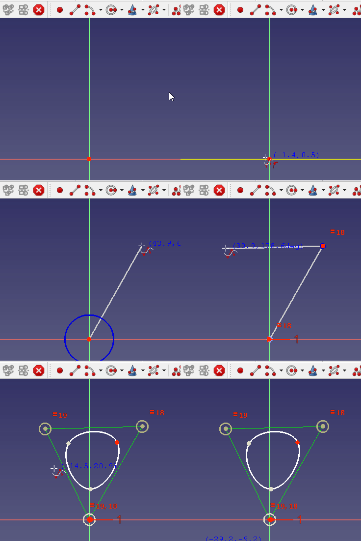
To create periodic B-splines (B-splines that form a closed curve), use the toolbar button Periodic B-spline. It is not necessary to set the last control point onto the first one because the B-spline will automatically be closed:
B-splines can also be generated out of existing sketch segments. To do this, select the elements and press the the toolbar button Convert Geometry to B-spline.
While creating a B-spline, its degree can be specified by pressing the D key. With this, the default to create a cubic B-spline if possible, can be overridden. introduced in version 0.20
Changing the Degree
To change the degree, select the B-spline and use either the toolbar button Increase B-spline degree or
Decrease B-spline degree.
Note: Decreasing the degree cannot revert a prior increase of the degree, see the Wiki page Decrease B-spline degree for an explanation.
Changing the Knot Multiplicity
The points where two Bézier curves are connected to form the B-spline are called knots. The knot multiplicity determines how the Bézier parts are connected, see the Wiki page Increase knot multiplicity for details.
To change the knot multiplicity, use the toolbar buttons B-spline increase knot multiplicity or
B-spline decrease knot multiplicity.
Note: Creating two B-Splines that are connected to each other will not unite to a single new B-spline. So their connection point is not a knot. The only way to get a new knot in an existing B-spline is to decrease the degree. However, you may get many new knots. Thus the better choice is to redraw the B-spline with more control points.
Changing the Weight
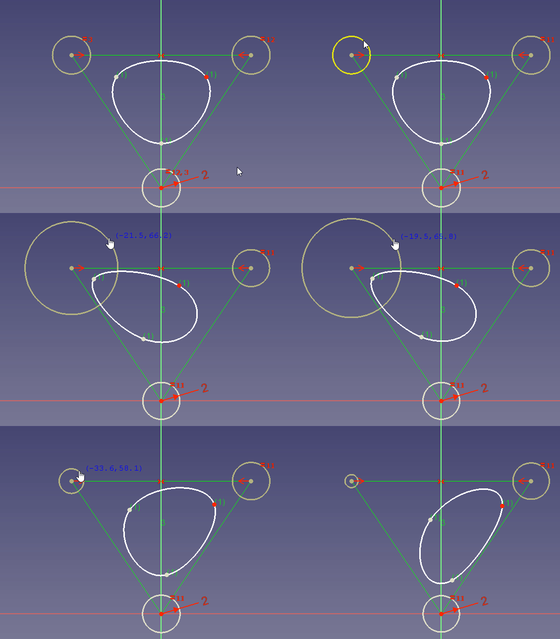
Around every control point you see a dark yellow circle. Its radius sets the weight for the corresponding control point. By default all circles have the radius 1. This is indicated with a radius constraint for the first control point circle.
To create a rational B-spline the weights have to be made independent. To achieve that you can delete the constraint that all circles are equal and then set different radius constraints for the circles.
If no radius constraint is set, you can also change the radius by dragging:
In the dragging example you see that a high weight attracts the curve to the control point while a very low weight changes the curve so as if the control point does almost not exist.
When you look at the creation function for non-uniform rational B-splines you see that a weight of zero would lead to a division by zero. Negative weights are theoretically possible but they are not supported. Therefore you can only specify weights greater than zero.
Editing Knots
New knots can be added using the B-spline insert knot button. introduced in version 0.20
A knot is deleted by decreasing it's degree to 0 (i.e applying decrease knot multiplicity when it's degree is 1).
Changing the parameter value of a knot is not yet supported.
Display Information
Since the form of a B-spline does not tell much about its properties, FreeCAD offers different tools to display the properties:
| Property | Toolbar button |
| Degree | |
| Control polygon | |
| Curvature comb | |
| Knot multiplicity | |
| Weights |
Limitations
At the moment (FreeCAD 0.19) there are some limitations when using splines you should know:
- You cannot set tangential constraints.
In this example
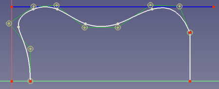
you want to assure that the spline touches the blue curve 2 times tangentially. This would be useful because the blue line could for example be the spatial border for your design. - You cannot insert a new control point between two selected existing control points. There is no other way than to redraw the spline.
- You cannot delete a control point. Also in this case you must redraw the spline
- You cannot create an offset curve for a B-spline using the tool Draft Offset.
Typical Use Cases
According to the properties of B-splines, there are 3 main use cases:
- Curves that start/end tangentially to a certain direction. An example for this is the motivation example above.
- Curves describing larger designs and providing the freedom of local changes. See this example below.
- Curves providing a certain continuity (derivative). See this example below.
Designing
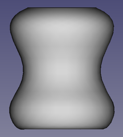
Take for example the case that you design a housing of a kitchen mixer. Its desired shape should look like this one:
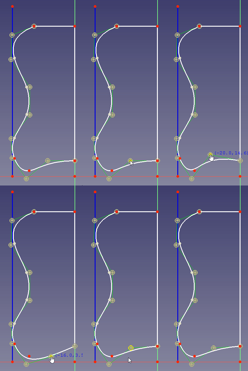
To define the outer form it is advantageous to use a B-spline because when you change a control point to change the curvature at the bottom, the curvature at the side and top will not be changed:
Continuity at Geometric Transitions
There are several cases where it is physically necessary to have a certain surface continuity at geometric transitions. Take for example the inner walls of a fluid channel. When you have a change in the diameter of the channel, you don't want to have an edge because edges would introduce turbulences. Therefore, like in the motivation example above, one uses splines for this purpose.
The development of the Bézier curves was initially triggered by the French car industry. Besides the saving of material and the reduction of the air flow drag, the look of the cars should also be improved. And when you look at the fancy design of French cars from the 60's and 70's you see that the Bézier curves gave car design a boost.
Let's take for example this task in the design of cars: The car fender should "look nice". Here is a basic sketch of our task:
"Looking nice" means that the (potential) customer looks at the fender and does not see unexpected light reflections and also no sudden changes in the reflection from the automotive paint at all. So what do you need to avoid changes in the reflections? Looking closely to the fender:
At the spatial area above the edge the intensity of reflected light is low (denoted by the red ellipse) because no light is directly reflected in the direction from the edge to the eye.
you see when there is an edge, there is a spatial area where the reflected light has less intensity and this is what you will notice when looking at the fender. To avoid this you need a continuous change in the slope of your surface elements. The slope is the first order derivative and as explained in section Basics, a second degree (quadratic) B-spline offers at every point a continuous first order derivative.
But is this really sufficient? At the point of geometric transition we have now at both sides the same slope, but the slope might change differently at both sides. Then we have this situation:
So we have also spatial areas in which the intensity of reflected light is different. To avoid this, we need at the geometrical point of transition also a continuity of the second order derivative and thus a cubic B-spline.
